We have all heard the dismissal: "LLMs are just predicting the next token." Technically true, but it's a bit like saying a conversation is just saying the next word. There is a lot going on under the hood, and this series is about the four ideas that do most of the work: weights, biases, loss functions, and gradient descent. Each one gets a part of its own, so do not worry if none of those words mean anything yet. They are the same core building blocks whether you are looking at the simplest possible model or at ChatGPT. That is why some of the most prominent voices in AI argue that the ability to predict should not be underestimated.

"It is the ability to make predictions about the future that is the crux of intelligence." Jeff Hawkins, On Intelligence
Prediction is everywhere
Humans have always been prediction engines. Our ancestors predicted weather patterns to hunt and farm. We predicted planetary motion to reach space. The ability to make accurate predictions about the future has been one of the defining advantages of human intelligence.
It is no surprise, then, that many academic fields have their own name for prediction: forecasting in meteorology, modeling in economics, projection in finance, extrapolation in statistics. And in machine learning, for reasons we are about to see, we use the term regression.

Galton and the origin of the word
The word "regression" in machine learning traces back to a Victorian-era polymath named Sir Francis Galton (1822–1911), a half-cousin of Charles Darwin. In 1886 he published a paper titled Regression Towards Mediocrity in Hereditary Stature.
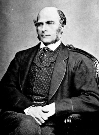
Galton was studying the relationship between parents' heights and their children's heights. To get one number per family he averaged the mother's and father's heights, a figure he called the mid-height, and you will see that word on every chart below. He focused specifically on families where the parents were extreme outliers, very tall or very short, and found something striking:
- Tall parents tended to have tall children, but not quite as tall as their parents.
- Short parents tended to have short children, but not quite as short as their parents.
In both cases the children's height regressed towards the mean, it pulled back towards average, rather than tracking the extreme of the parent. Galton called this regression to the mean, or regression towards mediocrity.
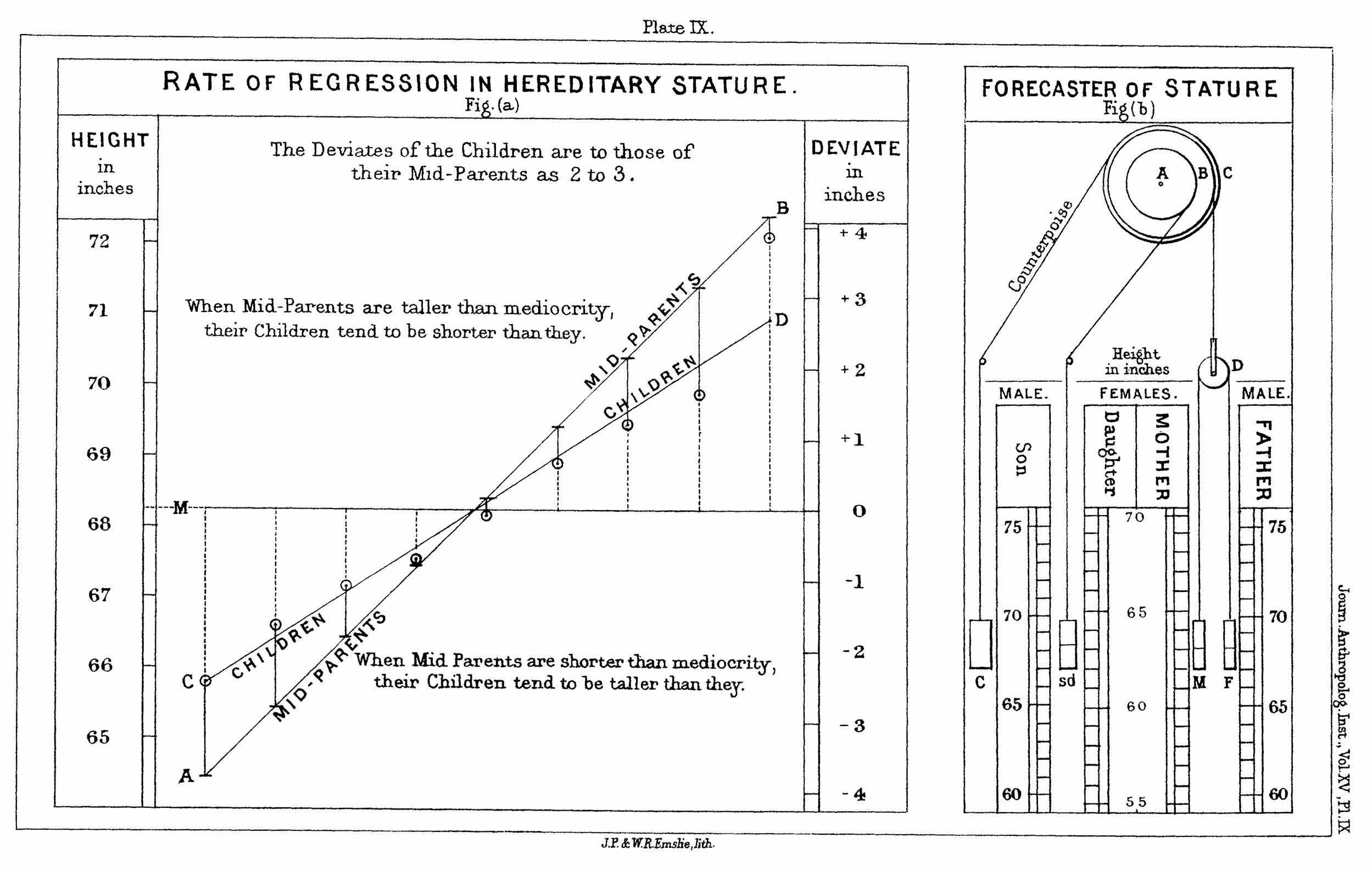
When he plotted the data, the children's heights fell roughly along a straight line. He called it the regression line, because the heights of each new generation tended to regress towards it.
Two words you will see on every chart from here on, and throughout the series. The thing we already know and use to make a prediction is the feature (here, the parents' mid-height). The thing we are trying to predict is the target (the child's height). Galton's dataset is just a list of feature values paired with the target value that went with each one.
Step one: the line is an average
Here is that plot redrawn, with the two axes spelled out, because getting these straight is most of the battle. The horizontal (x) axis is the parents' mid-height. The vertical (y) axis is the child's adult height. Every dot is one real family, placed where those two numbers cross.
Now look at what the line is actually doing. It does not pass through the dots, it passes through the middle of them. Some children turned out taller than the line says (green), some shorter (blue), and the two groups are almost perfectly balanced: 24 above, 22 below. Pick any parents' height, look straight up, and the line sits right in the thick of the children born to parents of that height, with about as many above as below.
That is the most useful way to think about a regression line: it is an average, drawn as a line. Not the average of everything lumped together, which would just be one flat number, but an average that slides as the input changes, tracking the typical child's height for each parents' height. It is the trend with the noise smoothed away.
Step two: an average you can predict with
Here is why that matters. An average of data you already have is a summary. But because this average is a line, it keeps going, including through heights where you have no data at all, and that turns a summary into a prediction.
A new couple walks in, and their mid-height is 72 inches. They are not one of Galton's dots; nobody has measured their child, who may not even be born yet. Trace the dashed path on the same chart:
- Find 72" on the horizontal axis. This is your known input, the feature.
- Go straight up until you hit the regression line.
- Read across to the vertical axis: about 70.5 inches. That is the prediction for the target.
That is a prediction, produced from a line and a number, for a family the model has never seen. And it is a sensible prediction precisely because of step one: the line is the average outcome for parents of that height, so 70.5" is the single best bet available. That move, from known input along the line to unknown output, is what every machine learning model in this series does. Everything that follows, weights and biases, loss functions, gradient descent, is machinery for finding the best possible line to do it with.
And a necessary word of caution: this is a prediction, and predictions can be wrong. Look at the hollow circles on the second chart, the actual children of 72-inch parents: they landed anywhere from about 68 to 73 inches. Not one of them was exactly 70.5. An average tells you where the middle is, never where any individual will land. Height depends on nutrition, luck, and thousands of genes the model knows nothing about. This gap between the confident line and the messy dots never goes away, no matter how sophisticated the model, and keeping it in mind is the difference between using a model well and trusting it blindly. (Later parts put numbers on that gap: it is exactly what loss measures.)
From Galton's paper to the linear model
Galton also worked out a rough formula to predict a child's height from their parents' mid-height:
child_height ≈ 0.66 × parent_mid_height + 23
Notice the shape of this formula. It looks like:
target = weight × feature + bias
This is the fundamental equation of linear regression. weight (here 0.66) controls the slope of the line: how much the target rises for every step of one in the feature, so how steeply the line tilts. bias (here 23) controls the intercept: where the line crosses the vertical axis, which is the value the target would take if the feature were zero.
These two values, weight and bias, are the two tuning knobs of any linear model. Given any weight and bias, you can reproduce any straight line. And once you have them, you can plug in a feature value you have never seen before to get a prediction.
That is exactly what machine learning does: it finds the values for weight and bias that best fit the data it is given, and then uses those values to predict targets for new inputs.
Three words you will see everywhere
Three more words that the rest of the series, and every conversation about machine learning, leans on. They are simpler than they sound.
- A model is the recipe that turns an input into a prediction. Galton's formula is a model. It is nothing more than a formula with some numbers in it, and those numbers (here the weight 0.66 and the bias 23) are called its parameters.
- A dataset is a collection of examples where you already know both the feature and the target: Galton's list of families with the parents' mid-height and the child's height for each one. The examples used to build the model are called the training data.
- Training is the process of working out the parameters from the training data. Galton did it by hand in 1886. Most of this series is about how a computer does it automatically, and that process turns out to be the same whether the model has two parameters or two hundred billion.
So when someone says "we trained a model on the data", they mean: we took a formula with blanks in it, and used a pile of known examples to fill in the blanks.
Try it: Galton's prediction machine
You can use Galton's 140-year-old formula right now. Slide the parents' mid-height below and the model predicts the child's adult height. Notice the regression-to-the-mean effect Galton discovered: very tall parents are predicted to have children shorter than themselves, and very short parents to have children taller than themselves, the prediction always pulls back towards the average.
predicted child height = 0.66 × 68.0 + 23 = 67.9 inches
Slide all the way to the right: parents with a mid-height of 76 inches get a predicted child of about 73 inches, tall, but below the dashed "same as parents" line. Slide to the far left: 60-inch parents get a predicted child of about 63 inches, above the dashed line. The two lines cross at roughly 68 inches, the population average, and every prediction is pulled towards it. That pull is regression to the mean, and the red line's two numbers, 0.66 and 23, are all the model needs to make a prediction for parents it has never seen.
What "linear" means
A linear relationship between a feature and a target means that as the feature increases, the target changes in a steady, predictable, straight-line way.
Some everyday examples:
- Average study hours and exam score: more hours, steadily higher scores (roughly).
- Years of experience and salary: more experience, steadily higher pay (roughly).
- Square footage and house price: bigger house, proportionally higher price (roughly).
The data will not lie perfectly on a line, there is always noise, but the underlying trend is linear enough that a straight line is a useful model.
Next: Weights, Bias, and the Linear Model where we make the weight and bias interactive so you can see exactly what they do to a line.